Summary: This tutorial provides you with guidelines on how to interpret the results of the differential expression (DE) analysis module of Oasis. The output consists of quality metrics and several different plots, such as principle component analysis (PCA), heatmaps and MA plots, which are useful for exploratory analysis of your data and results. It further includes an interactive web report that allows you to see which DE micro RNAs (miRNAs) target which genes, and gives you the opportunity to test for enrichment of various gene ontologies (GO) and pathways.
In addition, given that this module allows for the correction of expression values by including covariate information such as age and gender, this tutorial also includes an example that shows the improvement of results when carrying out DE analysis with covariates.
Most of the descriptions throughout this tutorial are based on the DE analysis output of the Renal cancer demo dataset (Osanto et al., 2012). For analysis with covariate information, the Alzheimer demo dataset (Leidinger et al., 2013) is used with covariate correction and without covariate correction.
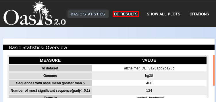
The first part of the output contains an overview table with quality metrics (Fig. ). This table reports the number of sRNAs with at least 5 mean reads for all biological conditions, the number of DE sRNAs at the 10% level of significance and the formula used to run the DE analysis.
Since not all sRNAs are effectively expressed for particular biological conditions, Oasis filters out such sRNAs to improve on the DE analysis. Therefore, Oasis only keeps sRNAs with an average of 5 reads for either condition.
Including the number of DE sRNAs at the lenient threshold of 10% will give you an idea of the overall proportion of sRNAs whose expression changes between biological conditions. So, for example, in Fig. , out of 400 sequences with support of at least 5 reads, 124 are DE at a 10% significance level, resulting in ~31% DE sRNAs, which is reasonable.
In addition to the Overview table, the output includes a principal component analysis (PCA) plot, heatmaps, MA plots and p-value distribution, which offer different visualisations of the sample similarities and the DE results.
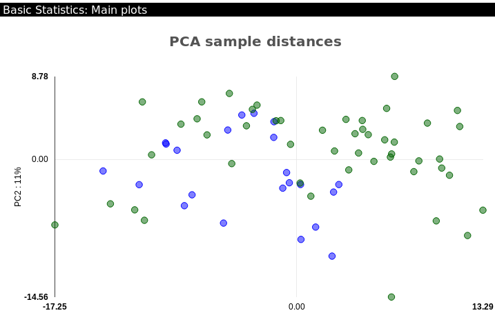
Principal Components Analysis (PCA) plot: (Figure ) this plot shows how well samples cluster together based on the similarity of their sRNA expression. Unlike the PCA in the sRNA Output Tutorial, this PCA distinguishes between samples based on their tested condition to see whether they are spatially clustered. In general, outliers and samples clustering in the wrong group will be an indication of few DE sRNAs, so removing such samples should improve on the DE analysis and generate more DE sRNAs. In the example renal data, we can see the samples cluster reasonably well based on their condition, indicating an expectancy of quite a few DE sRNAs (Fig. ). For more information on PCA plots, please refer to our sRNA Output Tutorial.
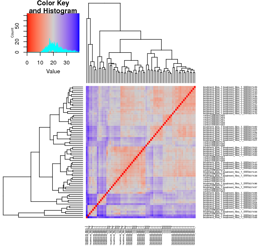
Heatmap: (Figure ) this plot depicts the similarities between samples, using a predefined colour convention. The first heatmap in the DE output corresponds to the matrix of Euclidean distances computed between all samples, where the distances are a function of the regularised-log (rlog) transformed counts of each sample. The heatmap contains an auxiliary "Color Key Histogram" on the top left to indicate the distances between the samples (red indicates distance 0 between same samples) and dendograms on the x and y axes show how samples cluster together. The renal data shows the treatment samples cluster well with each other, and the control samples occasionally cluster with the treatment samples, which should results in a reasonable amount of DE sRNAs (Fig. ).
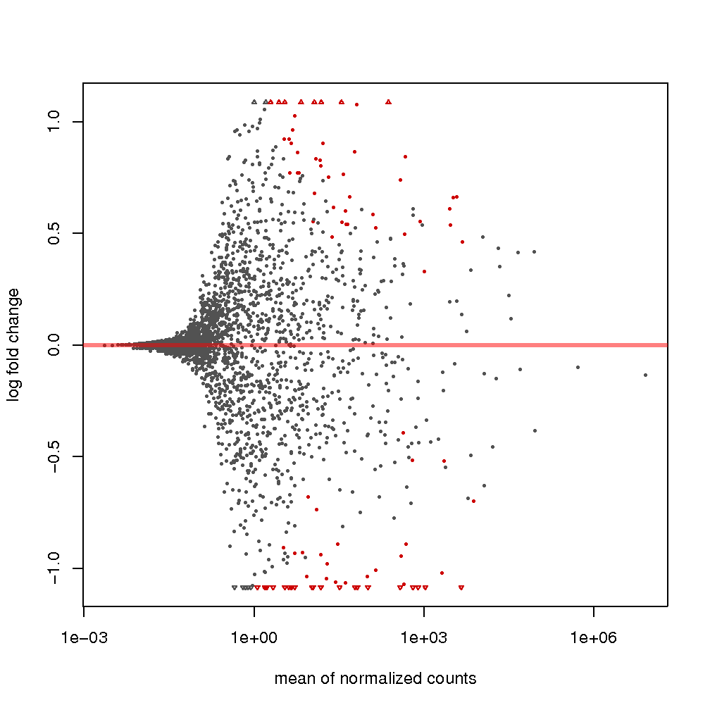
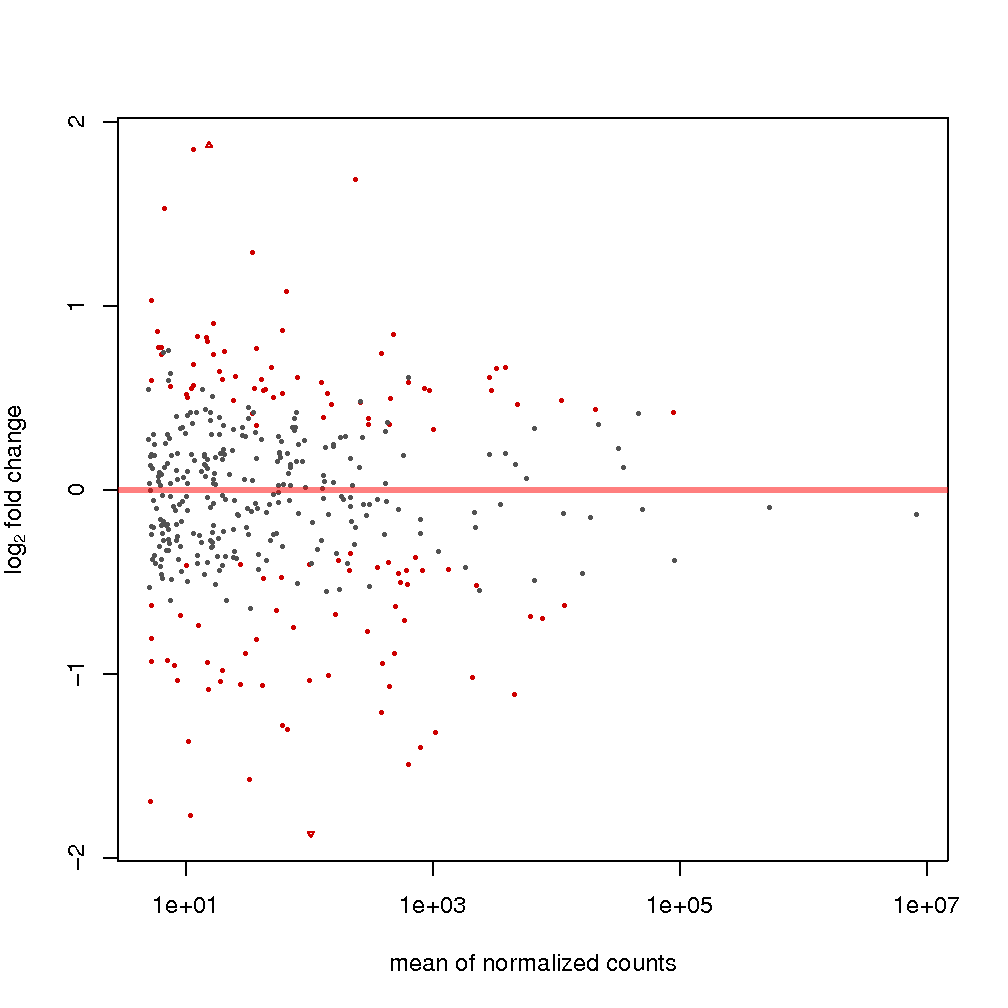
MA plots: MA plots are a particular instantiation of the method proposed in (Altman & Bland, 1983), which consists of graphically representing the agreement or disagreement of applying two experimental conditions according to some variable of interest. The method consists of plotting the recorded difference in the value of the variable as a function of the average value of such variable when applying the experimental conditions. In the particular case of DE analysis, the variable of interest is the expression level transformed by log2. As such, the dependent variable is the log2 fold change of the expression, and the independent variable is the mean expression. More information on the interpretation of this plot can be MA found plots in the DESeq2 manual (Love, Huber, & Anders, 2014). in the output show expression changes, attributable to applying the treatment condition as a function of average expression. The assumption is that in a well-carried experiment, the expression of most sRNAs between control and treatment conditions should remain constant, while only several of them would be considerably different. For example, see figures and .
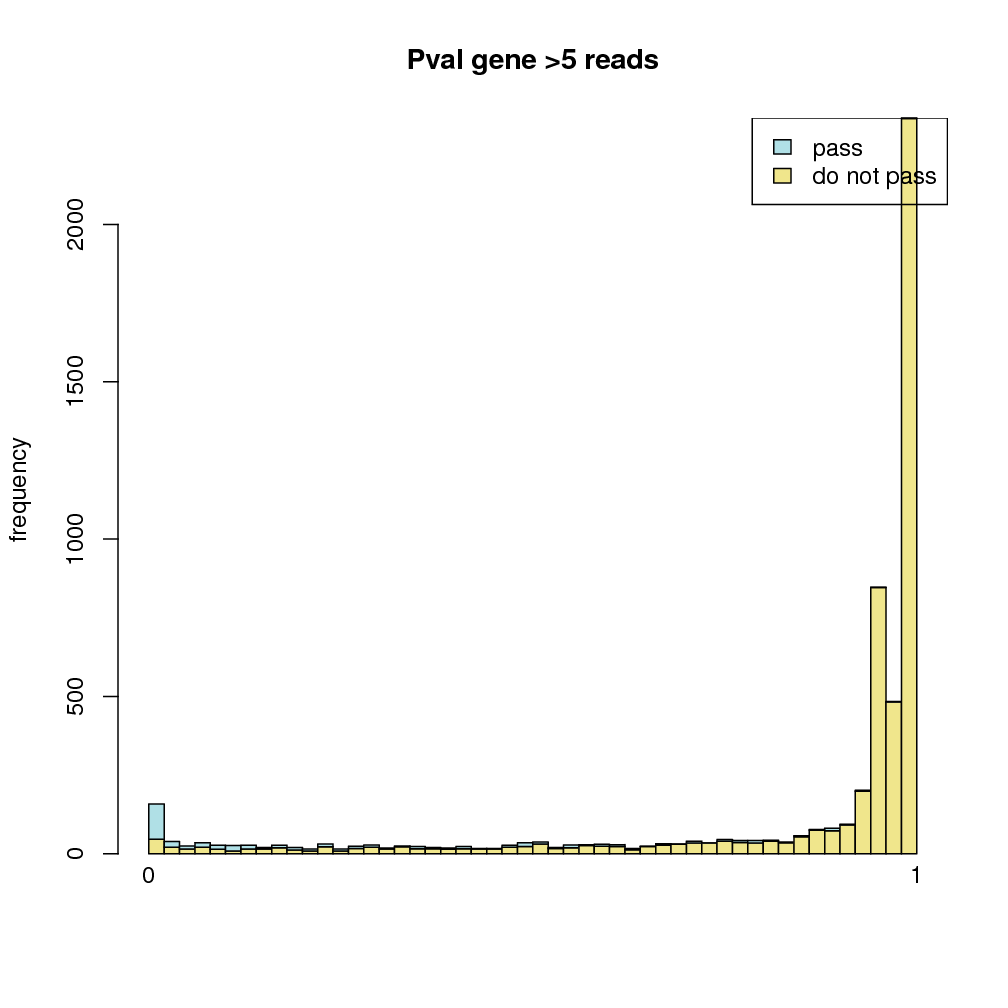
PValue distribution: in order to see the connection between the significance of sRNAs among different conditions and their expressions, the distribution of p-values is plotted for sRNAs that did or did not pass the filtering criteria (5 reads on average per condition). This plot is useful to see how many sRNA have a statistically significant p-value, but are not supported by enough evidence (read coverage) to be considered as such. In the case of the renal data, while many sRNAs do not seem to pass the filter criteria, it is mostly in the higher p-values, while lower p-values are more associated with sRNAs that pass the filtering criteria. Therefore, the expected correlation between low p-values and high sRNA coverage is clear in the renal data. The p-value distribution is depicted in figure .
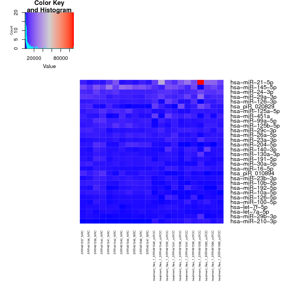
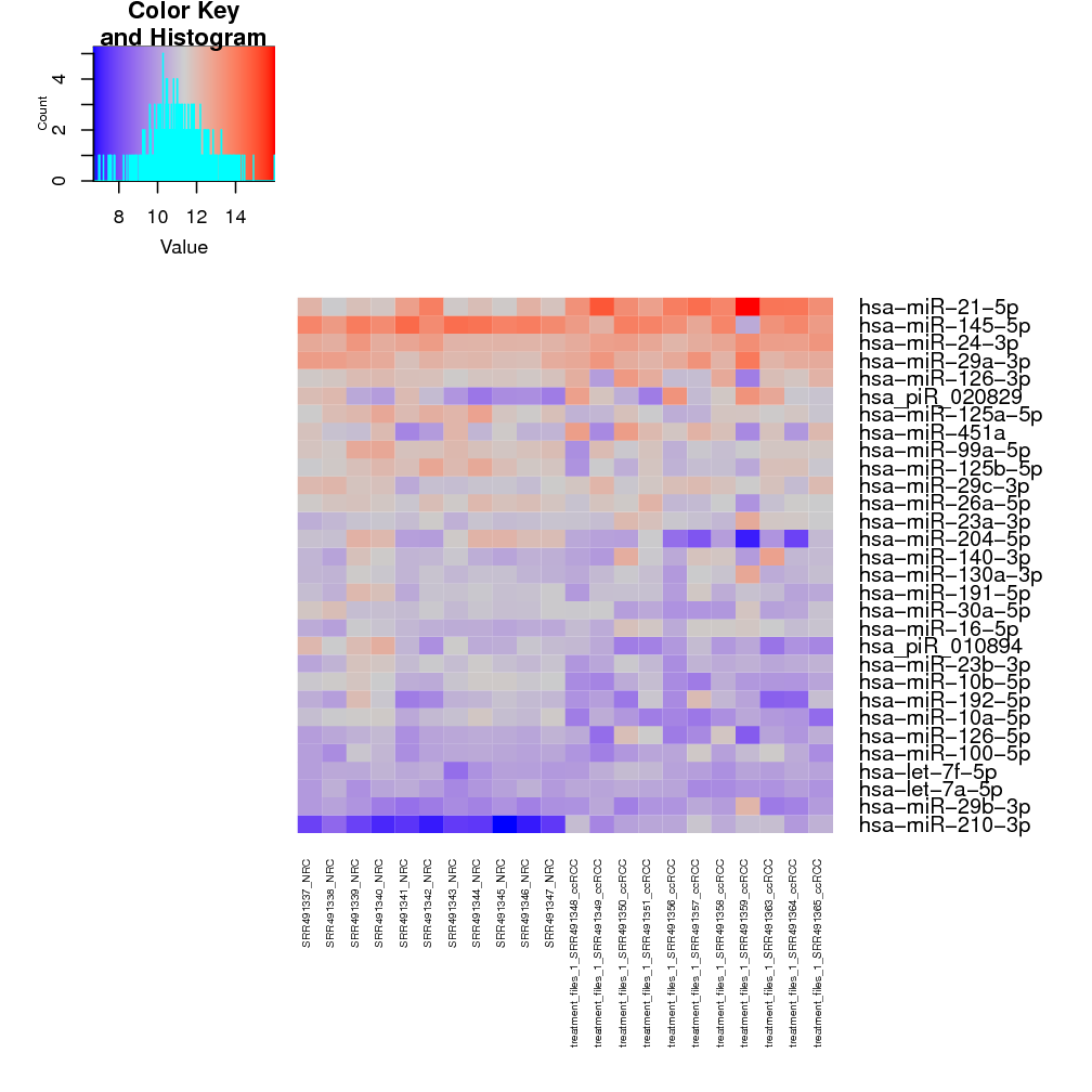
Top 30 most expressed sequences: these 2 heatmaps show the top 30 most expressed sRNAs from raw counts and rlog transformed counts. For the renal cancer demo data, a single sRNA with massive raw counts (red square) overshadows all other sRNAs with somewhat lower expression (blue squares) (Fig. ), while the rlog transformed counts for the sRNAs are spread across a reasonable scale (smooth flow from low expressions in blue to high expressions in red; Fig. ). This suggests that the rlog transformation normalises the data in such a way that the change in expression is gradual, not drastic like in the raw counts.
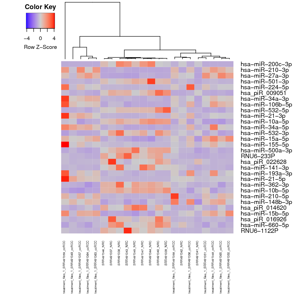
All significant sequences: this heatmap contains the top 30 most significant sRNAs with adjusted p-values below 0.1, as well as the sample clustering based on the expression of those sRNAs alone. For the renal data, while the samples had an incomplete clustering to “control” and “treatment” groups when plotting a heatmap for all sRNAs (Fig. ), NRC samples (representing control samples) still show mixed clustering with ccRCC samples when using a subset of top 30 most significant sRNAs (representing treatment samples) (Fig. ).
Apart from the statistical plots, the Oasis DE module returns an interactive web table that contains detailed information on each sRNA, and allows for the functional enrichment analysis of target sRNAs. To access this information, press the option "DE results" at the top of the HTML page (Fig. , red box). A new web page will open (Fig. ), containing two functional parts: functional analysis options (Fig. , blue box) and a table of all DE analysis results for the sRNAs (Fig. , red box).
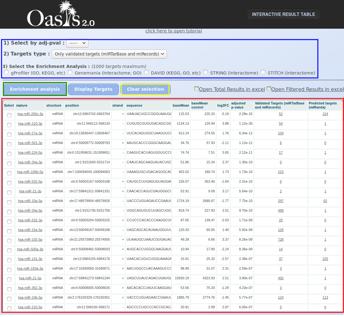
Within the table, columns “mature”, “structure”, “position” and “strand” indicate the name of the reported sRNA, the sRNA species it belongs to (for elaboration on sRNA species, see the sRNA Output Tutorial) and its position and strand, respectively. The columns “baseMean” and “baseMean control” represent the mean expression values for each condition. In the case of multiple treatment groups, just the “baseMean control” column is included. “log2FC” and “adjusted p-value” follow suit with the log2 fold-change in expression between conditions and the adjusted p-value, respectively. Finally, “Validated Targets” and “Predicted Targets” indicate how many validated and predicted gene targets are linked to the sRNA. Clicking on one of the target entries will show a list of the gene targets as gene names.
The enrichment analysis of Oasis allows the user to select specific miRNAs (either manually or by filtering based on adjusted p-value threshold), and use the associated genes to find which gene ontology (GO) categories, KEGG pathways or protein-protein interactions are enriched for them.


Finally, submit your enrichment analysis by clicking the Enrichment analysis button (Fig. , green box). You may submit jobs to multiple enrichment tools at once, but consider that a new browser window will open for each tool you use, and it will take longer to run. If the links do not open, try disabling your popup blocker.
Notes:When having a set of DE genes associated with particular miRNAs, the most direct way to derive some biological context from them is to run an enrichment analysis. This analysis finds particular biological terms or pathways which contain have a strong representation of DE genes within them. There are various tools to do such test, and here are several which are available through Oasis:
For covariate-based DE analysis, we have a demo Alzheimer's dataset (Leidinger et al., 2013). First of all, it is important to mention that this dataset contains 3 outlier samples (SRR837453, SRR837503 and SRR837506) (see sRNA detection results for the Alzheimer’s dataset). As such, those samples are removed from the DE analysis, resulting in 22 control and 45 Alzheimer's samples. Second of all, using the covariate table as mentioned in the Oasis DE tutorial, the analysis can be run with the covariate information or without it. This means the analysis is run once with the samples only, and once with the covariate table and the formula ~Gender+Age+DiseasePheno (for more details, see the Oasis DE tutorial). When comparing both results, they seem fairly similar, where the analysis with covariates has 179 sRNAs after coverage filtering (minimum 5 reads on average) and the other analysis has 178 sRNAs after coverage filtering. In addition, the analysis without covariates has 70 DE sRNAs, whereas the other analysis has 67 DE sRNAs. The reason 3 DE sRNAs without the covariate information are not DE with the covariate information is because those sRNAs are DE due to the variations of gender or age between the different samples, but the distinction between the disease phenotype (AD or C) is actually non-significant when the gender and age variations are corrected for. Therefore, the covariate information allows removing false positive DE sRNAs, which are only DE due to factors not relating to the actual tested conditions.