Overall Quality Control (QC)
This part will guide you how to assess the quality of your data from the sRNA Detection analysis. Various plots and metrics in this output will provide you with insight into the overall technical and biological quality of your samples.
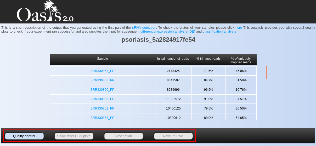
The first thing you will see when opening the page is the Summary Statistics table, containing information on the total number of reads, percentage of trimmed reads (adapter trimming), and percentage of uniquely aligned reads per sample (Fig. ). In general, low percentages of trimmed and/or uniquely mapped reads indicate problematic samples. If there are only few samples with such low quality indicators, they can be treated as outliers and therefore be removed from downstream analyses. Nevertheless, when many/all of your samples show low percentages of trimmed or mapped reads, the adapter or reference genome you selected, respectively, may have been non-corresponding for the input samples. Alternatively, it is possible that your sample was contaminated with foreign genomic material, or it might have a lot of repetitive short sequences.

In addition to the summary statistics table, you will notice a menu below it, showing multiple buttons (Fig. , red box). Pressing each of the buttons will show you a different set of results.
- Quality control: Pressing this button will show you various
interactive plots of overall sample qualities:
-
Principal component analysis (PCA) plot: the PCA plot gives you an overview of
the sample similarities by showing how well samples cluster with each other
based on their sRNA expression. In brief, the PCA plot shows two leading
principal components (PCs) of the data in the x and y axes, with the
percentages of variance “explained” by each of them next to the equivalent PC.
The PCA plot can be used to detect outlier samples, which can negatively affect
the detection of differentially expressed (DE) sRNAs (increasing the variance).
As mentioned before, such outliers should be removed for downstream analyses.
As there are no clear outliers in the PCA plot for the psoriasis data (Fig. ),
we can conclude this data has good quality in terms of general variance between
the samples. In order to show you what an outlier in the PCA plot looks like,
Fig. shows the PCA plot of our Alzheimer’s demo dataset (Leidinger et al.,
2013), where samples SRR837503, SRR837506 and SRR837453 are clear outliers.
The PCA plot in the output also has an interactive feature, where the sample
name appears for a particular point when the mouse is moved unto it.
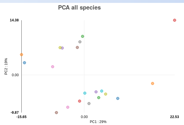
Figure : PCA plot for psoriasis demo data. 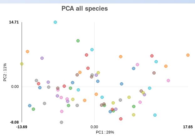
Figure : PCA plot for alzheimer demo data. -
Trimmed reads: these interactive bar plots show how many reads are
filtered for being too short or too long. By pressing the different
buttons at the top, the bars can be shown (solid button) or hidden
(hollow button). In addition, when you move the mouse unto a bar, the
plot shows the approximate number of reads that are too long or short
for a particular sample (using “k” and “M” to indicate thousands and
millions of reads, respectively). For the psoriasis data, the minimum
read length used was 15 bp and the maximum read length used was 40
bp, and while many reads were filtered out for being shorter than 15 bp,
no reads were filtered for being longer than 40 bp (Fig. ).
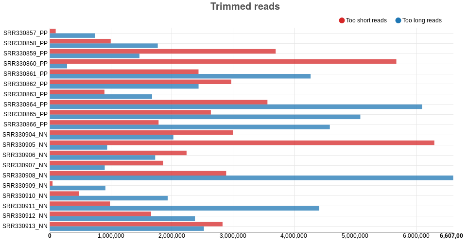
Figure : Trimmed reads of the Psoriasis data set. -
Reads per species: sRNAs are grouped into various species, including
micro RNA (miRNA), piwi RNA (piRNA), small nucleolar RNA
(snoRNA), small nuclear RNA (snRNA) and ribosomal RNA (rRNA).
As such, the reads may be associated with any of those sRNA species,
and the equivalent plot shows the percentage of reads associated with
each of the species. Similar to the “trimmed reads” barplot, bars can be
shown or hidden, and the information of each bar is shown when the
mouse is moved unto it. For the psoriasis data, the samples have a
larger proportion of miRNA reads than reads associated with the other
species (Fig. ).
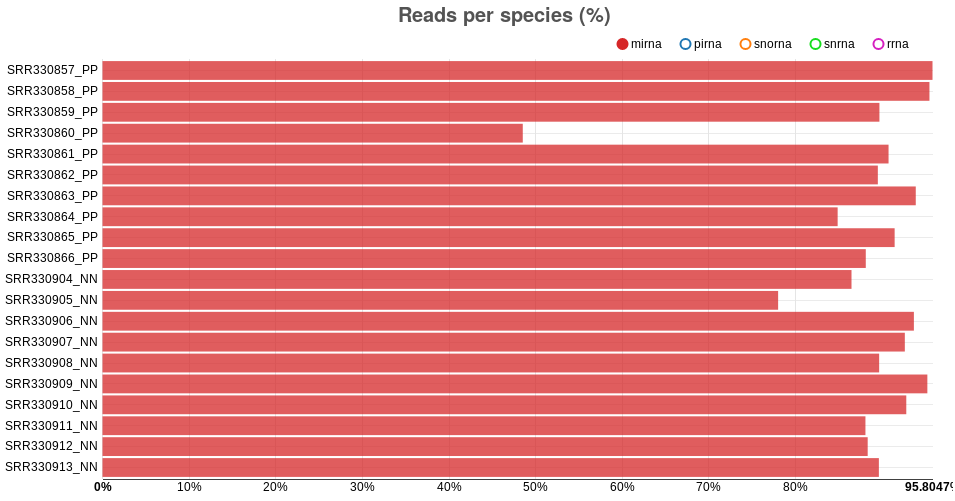
Fig. : number of reads per sRNA species in psoriasis data -
Mapped reads: this barplot shows how many reads are initially
present for each sample, how many are kept after trimming and length
filtering, and how many are uniquely mapped to the reference genome.
Similar to the “trimmed reads” barplot, bars can be shown or hidden,
and the information of each bar is shown when the mouse is moved
unto it. The psoriasis data shows a relatively small difference between
the initial number of reads and the reads kept after filtering, indicating
few reads have been discarded after trimming. However, the number of
mapped reads is much smaller compared to the initial number of reads.
Nevertheless, sRNA-seq samples are known for having considerably
small mapping rates, and for such samples, such patterns are
reasonable (Fig. ).
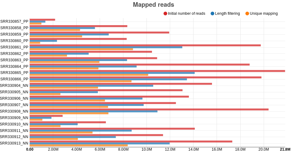
Figure : Number of reads as different steps of the sRNA detection analysis on psoriasis data
-
Principal component analysis (PCA) plot: the PCA plot gives you an overview of
the sample similarities by showing how well samples cluster with each other
based on their sRNA expression. In brief, the PCA plot shows two leading
principal components (PCs) of the data in the x and y axes, with the
percentages of variance “explained” by each of them next to the equivalent PC.
The PCA plot can be used to detect outlier samples, which can negatively affect
the detection of differentially expressed (DE) sRNAs (increasing the variance).
As mentioned before, such outliers should be removed for downstream analyses.
As there are no clear outliers in the PCA plot for the psoriasis data (Fig. ),
we can conclude this data has good quality in terms of general variance between
the samples. In order to show you what an outlier in the PCA plot looks like,
Fig. shows the PCA plot of our Alzheimer’s demo dataset (Leidinger et al.,
2013), where samples SRR837503, SRR837506 and SRR837453 are clear outliers.
The PCA plot in the output also has an interactive feature, where the sample
name appears for a particular point when the mouse is moved unto it.
- Show other PCA plots: pressing this button will show you PCA plots for different sRNA species. While they are not interactive, they work on the same principle as the previous PCA plot, but using expressions of reads belonging to particular sRNA species.
- Description: pressing this button will show you an online version of this tutorial.
- Novel miRNA: pressing this button will show you information on novel miRNAs that have been predicted during the sRNA Detection analysis. This section contains a table with a provisional ID, a score given by the miRDeep2 software, and information regarding the number of reads involved and the consensus sequence. Clicking on the provisional ID opens a PDF file with additional information, including an image of the folded miRNA structure and the sequences contributing to its consensus sequence.
Individual Sample Quality Control
The output of Oasis’ sRNA Detection module also allows you to look at each sample in more detail. By clicking on a sample name in the summary statistics table (for example, SRR330857 in Fig. ), you will access detailed information on the sample in a new browser window (Fig. ). This part of the tutorial will explain the different plots and tables for the individual samples as you would access by clicking on a sample name.
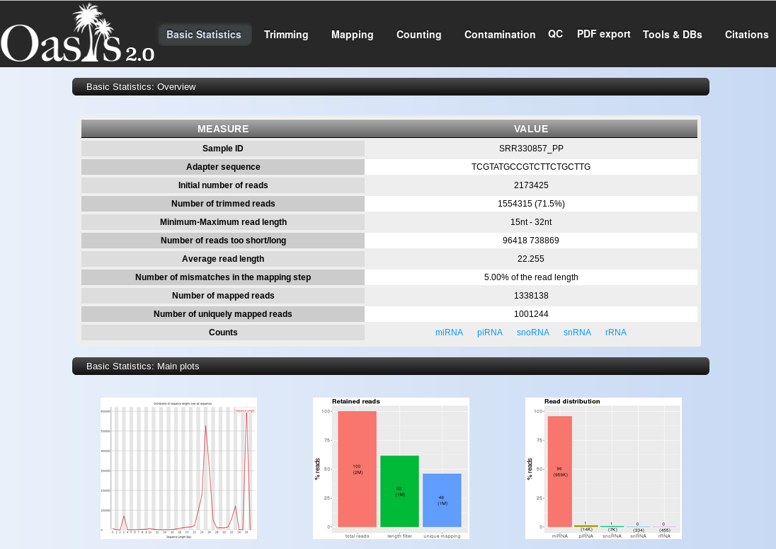
- Basic statistics Overview: the single sample QC output gives the most important information on its entry page, namely a table with expanded statistics including initial number of reads, number of trimmed reads (adapter removal), maximum and minimum read lengths (used for length filtering of reads, as set in the sRNA Detection analysis), number of reads too short or long (depending on maximum and minimum lengths), average read length (after filtering), number of mismatches allowed for mapping (as set in the sRNA Detection analysis), number of all mapped reads, and number of uniquely mapped reads. Read-length distribution plot: this plot shows the size distribution of
- Read-length distribution plot:
this plot shows the size distribution of
reads after adapter removal and before length filtering. This plot should
contain a peak centered at 19-25 bp that represents miRNAs and other
small RNAs like piRNAs. An additional peak at the maximum length is also
possible. In the optimal case, you will see a strong peak at 19-25 bp and
little to no reads below the minimum length or above the maximum
length. In the case of the psoriasis sample SRR330857, no reads have
length above 36, and few reads have length below 15, so it is a relatively
high quality sample.
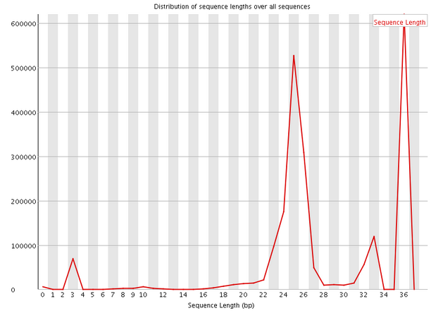
Figure: : Read length distribution plot -
Filtering barplot: this plot shows the total numbers and percentages of
initial input reads (total reads), reads left after length filtering (length
filter) and reads that map uniquely to the genome (unique mapping) (Fig.
). For each bar, the percentage appears in the middle of the bar and the
number shown in brackets is the number of reads in thousands (‘k’) or in
millions (‘M’). The “length filter” bar shows reads left after adapter
removal (trimming) and filtering for reads that are too short or too long.
The “unique mapping” bar shows reads that are uniquely map to the
genome. High length filter and unique mapping percentages indicate good
sample quality in principle, but those numbers can still vary greatly
depending on the organism, tissue, cell-type, and protocols used.
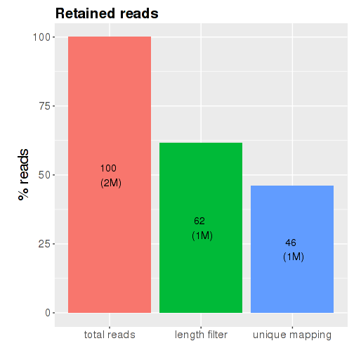
Figure : Read filtering barplot - sRNA species barplot:
this plot shows the percentage (and total
number) of reads that have been assigned to specific sRNA species (Fig.
). Since miRNAs are prominently the most prevalent specie, results will
usually show a high number of miRNAs and few of the other sRNA
species. Nevertheless, the exact distribution of reads over the different
sRNA species will depend on the organism, tissue, cell-type, or protocols
used, and can vary greatly.
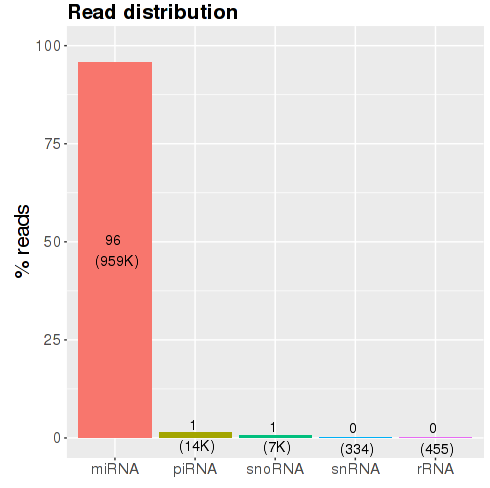
Figure sRNA classes barplot Count files and subsequent analyses
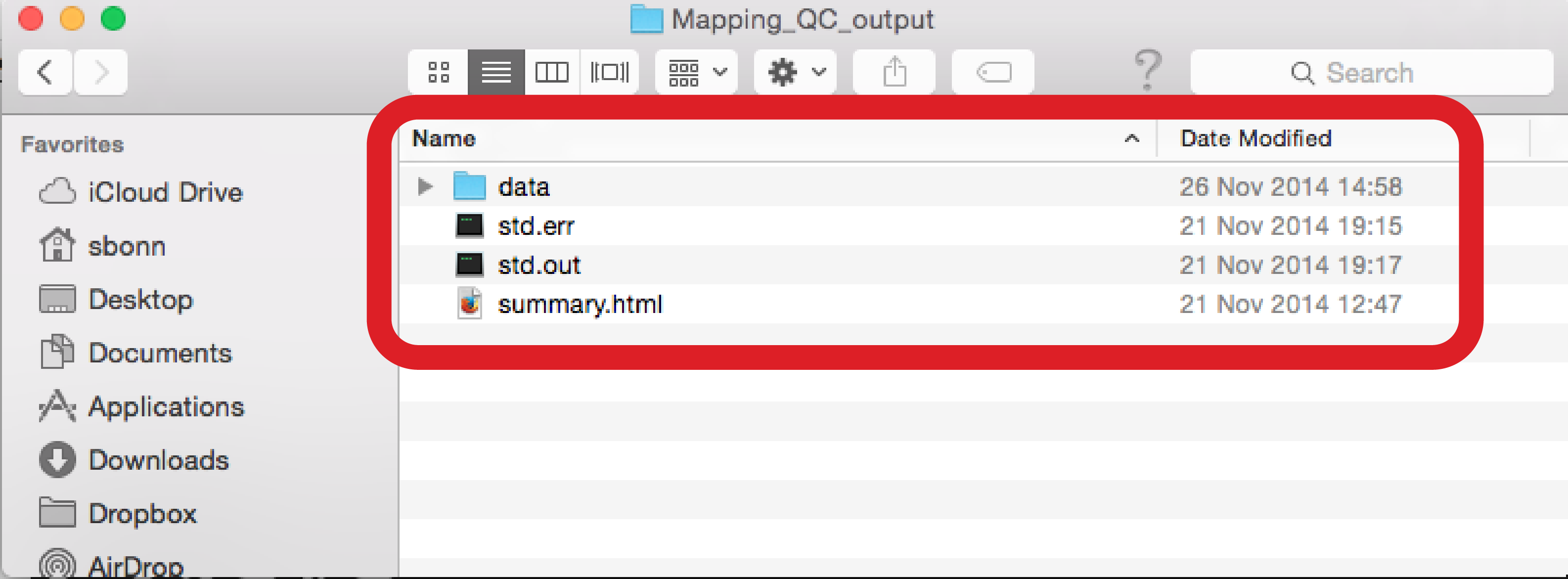
Within the output directory (Fig. ), you will notice a directory “data”. Within this directory, you will find a directory “counts”, which contains text files with the sample names and the ending “allspeciesCounts”, indicating those are count files for all known sRNA species, as well as novel, predicted miRNAs, found for each sample (Fig. ). Each count file contains a particular sRNA ID and the number of reads associated with it, and those files are uploaded to the downstream analyses modules, i.e. the differential analysis or the classification. As mentioned before, having the quality module separated from the downstream analyses gives you an opportunity to look at the sample qualities, determine if any of them are of bad quality, and leave their corresponding count files out of the downstream analysis.
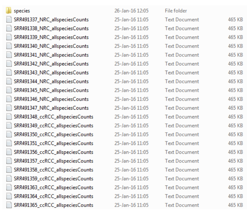
Figure :Directory listing with allspeciesCounts files Other information
If you are interested in the details of the sRNA Detection analysis, please read the original publication (Capece et al., 2015). If you use the original Oasis publication, please cite it, as citations are our currency and allow us drive the development of Oasis further. In case you want to give us feedback, please send an e-mail to oasis@dzne.de. We are happy to receive your criticism and suggestions as this will make Oasis a better analysis tool. With this we leave you to your analysis and wish you god-speed from the Oasis team.References
- Capece, V., Garcia Vizcaino, J. C., Vidal, R., Rahman, R.-U., Pena Centeno, T., Shomroni, O., … Bonn, S. (2015). Oasis: online analysis of small RNA deep sequencing data. Bioinformatics, 31(13), 2205–2207. http://doi.org/10.1093/bioinformatics/btv113
- Joyce, C. E., Zhou, X., Xia, J., Ryan, C., Thrash, B., Menter, A., … Bowcock, A. M. (2011). Deep sequencing of small RNAs from human skin reveals major alterations in the psoriasis miRNAome. Human Molecular Genetics, 20(20), 4025–40. http://doi.org/10.1093/hmg/ddr331
- Leidinger, P., Backes, C., Deutscher, S., Schmitt, K., Mueller, S. C., Frese, K., … Keller, A. (2013). A blood based 12-miRNA signature of Alzheimer disease patients. Genome Biology, 14(7), R78. http://doi.org/10.1186/gb-2013-14-7-r78